Basics operations, Functions, and Looping in R
There are multiple arithmetic operations in R, such as Addition, Multiplication, Subtraction, and Division. You can store numerical value in a variable and do basic operations or simply write numerical value and calculate it.

Operations:
R is a powerful calculator; you can use a wide range of numerical computations and calculations in R.
There are multiple arithmetic operations in R, such as Addition, Multiplication, Subtraction, and Division. You can store numerical value in a variable and do basic operations or simply write numerical value and calculate it.
Addition(+):
A=265; B=657; A+B
Output: [1] 922
A+25
Output:[1] 290
Subtraction(-):
A=640; B=345; A-B
Output: [1] 295
A-50
Output: [1] 590
Multiplication():
A=48; B=34; AB
Output: [1] 1632
412*500
Output: [1] 206000
Division(/):
To get quotient
A=48; B=8; A/B
Output: [1] 6
50/4
Output: [1] 12.5
Modulus Returns Remainder Division(%%):
A=48; B=8; A%%B
Output: [1] 0
50%%4
Output: [1] 2
Squaring Number:
A=25; A^2
Output: [1] 625
Or
25^2
Output: [1] 625
Square Root:
2^(1/2)
Output: [1] 1.414214
Or we can use function sqrt() to get the square root of the number.
sqrt(2)
Output: [1] 1.41421
Function:
In mathematics, a function produces one or more outputs from one or more variables (or inputs). In R, functions operate analogously.
There are two types of functions in R, Built-in Function and User-defined Function.
Built-in Function:
R has a large number of Built-in functions and also user can create their functions.
In R, you must put the function name followed by its argument values surrounded in parentheses and separated by commas to call or invoke a built-in (or user-defined) function.
Here I illustrate the use of the ‘seq’ function, which generates arithmetic sequences.
#Creating a sequence of 2 to 20 by a difference of 2.
> seq(from=2, to=20,by=2)
Output: [1] 2 4 6 8 10 12 14 16 18 20
So in the above function(seq()), there are three arguments which are ‘from’,’to’, and ‘by’. In this function, some arguments are optional and have predefined values. For example, if we remove ‘by’ from function seq() it will generate the sequence with a difference of 1.
> seq(from=2, to=20)
Output: [1] 2 3 4 5 6 7 8 9 10 11 12 13 14 15 16 17 18 19 20
There is a standard parameter order for each function. Arguments do not need to be named if they are provided in this order, but you are free to submit arguments out of order as long as you name them using the format argument name = expression.
> seq(2,10,2)
Output: [1] 2 4 6 8 10
Another example of a Built-in Function mean(), the mean of a given vector x.
> x=c(2,8,6,4,12,21,14,32,24)
> mean(x)
Output: [1] 13.66667
User-defined Function:
Syntax:
function_name=function(argument1,argument2,..){
Function body
…
}
The function name is the actual name of the function as we stored the vector name in the R environment. An argument serves as a stand-in. Whenever a function is called, an argument is passed with a value. Arguments are optional; therefore, a function may not require any of them. Argument default values are another possibility. The function body contains all expressions and a collection of statements that define what the function does.
Here are some examples of User-defined functions.
Let's get a square of any number through a User-defined function.
#Creating a function to get the square of any number.
Square<-function(a) {
b=a*a
print(b)
}
In the above example Square() is the name of the User-defined function and ‘a’ is an argument. To call the User-defined function write the function name with the argument.
> Square(8)
Output: [1] 64
You can create a function without any argument. Here is an example of a function without argument.
# Table of 13
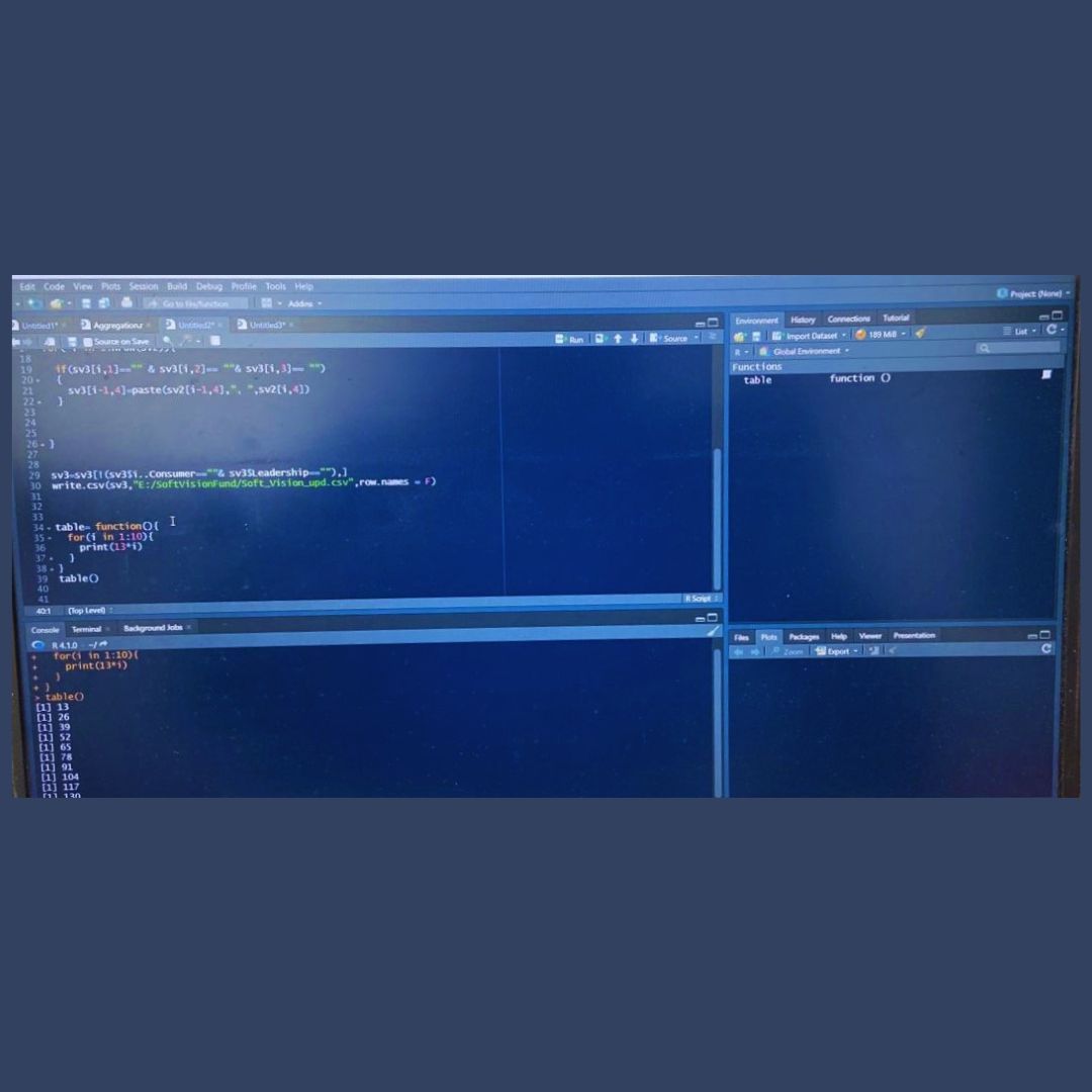
table= function(){
for(i in 1:10){
print(13*i)
}
}
> table()
Output: [1] 13
[1] 26
[1] 39
……
R allows functions to take any number of parameters, including none at all. Even if there are no arguments needed, parentheses are always necessary when calling a function. Simply typing the function name causes R to type out the function's "object," which is the program that defines the function. Typically, we only cover the most crucial or frequently used choices when describing functions. You should utilize the integrated help feature for comprehensive definitions.
Loop:
R programming requires control structures to execute blocks of code multiple times. Loops are one of the most basic and powerful programming concepts. A loop is a control statement that allows a statement or series of statements to be executed multiple times. The word "loop" means to cycle or repeat.
Loop creates a query in a looping structure. If action is required in response to this query, the action is taken. The same query is repeated over and over until more actions are taken. Each time a query is issued within the loop is called an iteration of the loop. A loop has two components: the control statement and the loop body. Control statements conditionally control the execution of statements, and the loop body consists of a series of statements to be executed.
There are three types of loops in R programming.
· For Loop
· While Loop
· Repeat Loop
Looping with ‘for’:
A for loop is often used to iterate over the elements of a sequence. This is the input control loop. In this loop, the test condition is tested first and then the main part of the loop is executed. If the test condition is false, the loop body is not executed.
Syntax:
For (value in sequence) {
Statement
….
}
# Creating a square for the given vector
X=c(4,9,6,12,14)
for (i in X) {
b=i^2
print(b)
}
Output:
[1] 16
[1] 81
[1] 36
[1] 144
[1] 196
So, this is an example of a ‘for loop’ where the loop is iterated over a number in vector X and displayed square of every number of vector X.
Looping with ‘while’:
Syntax:
While (logical expression) {
Expression_1
…
}
A while loop is more basic than a for loop, as you can always do. While loop is based on a logical expression. It will run a statement or set of statements until the given condition became false. It is also an entry-controlled loop because it tests the condition first and after that executes the body of the loop. The loop body would not be executed if the condition is false.
Here is the example of getting factorial of any number through a while loop. Let the number be 6.
n=6; fact=1; i=1
while(i<=n){
fact=fact*I; i=i+1
}
> fact
Output: [1] 720
So this is the example of a while loop where the loop is iterated until and unless ‘i’ is equal to or less than n(6).
Looping for ‘Repeat’
It is a straightforward loop that repeatedly executes the same statement or a set of related statements up until the stop condition is reached. A programmer must expressly include a condition within the loop's body and utilize the declaration of a break statement to end a repeat loop since it lacks a conditional clause. The repeat loop will loop indefinitely if there is no condition in the body of the loop.
Syntax:
repeat {
commands
if (condition){
break
}
}
Here is the example of a repeat loop that iterates five times “Hi” “There”.
Word=c("Hi", "There"); count=1
Repeat {
print (Word)
count=cnt+1
if(count>5)
break
}
Output:
[1] "Hi" "There"
[1] "Hi" "There"
[1] "Hi" "There"
[1] "Hi" "There"


